Why Accuracy and Precision Matters
To confidently measure the rates of degradation mechanisms occurring in a cell, more than an order of magnitude better accuracy and precision is needed than the actual rates being measured. For example, in modern commercial cells, rates of Capacity Fade and Charge Endpoint Capacity Slippage are on the order of C/10,000-C/50,000, or 100ppm-20ppm of C-rate. This means that cell cycling equipment must have on the order of 1-10s of ppm measurement accuracy to achieve adequate values of these metrics to make early, informed, and confident decisions.
Charge Endpoint Capacity Slippage is nearly impossible to measure on standard cell testing equipment. To elaborate, first consider Capacity Fade, which is quantified by measuring over subsequent cycles. Capacity Fade has a cumulative effect, meaning that each cycle’s Capacity is affected by the previous cycle’s Capacity Fade. If a low accuracy cycler has a consistent bias towards overcounting Discharge Capacity, the cycler will report the individual cycle Discharge Capacities to be higher than reality by some amount. However, taking the difference between those Discharge Capacities effectively removes this bias, and thus Discharge Capacity Fade is not significantly affected by poor accuracy. If a cycler has poor precision, there may be some noise in the measurement of Discharge Capacity Fade, but over multiple cycles, the cumulative nature of Capacity Fade means a trend will be clear as the Discharge Capacity will decrease, thus an average Capacity Fade rate can be interpreted.
However, Charge Endpoint Capacity Slippage relies on both charge and discharge capacities to be accurate. For example: If a cycler has an accuracy bias that undercounts charge capacity and overcounts discharge capacity, the charge endpoint may move much slower or even backwards on one channel, while the next channel with an identical cell has the opposite bias; significantly biasing the charge endpoint to higher capacity. Thus why accuracy and precision of a cycler must therefore be at least an order of magnitude better than the rate of slippage-based mechanisms in order to use Charge Endpoint Capacity Slippage as a metric.
In Figure 9, for example, the cells tested were ~ 1000 mAh, tested at C/10 (100 mA). The rate of slippage-based mechanisms in Electrolyte 2 can be approximated as the amount of capacity slippage over the length of the cycle (0.0002 Ah / 20 h = 10 uA or 100ppm of the applied current). Therefore, to accurately track these endpoints, a cycler requires current measurement accuracy on the order of 10 ppm. Only NOVONIX UHPC systems have been shown to perform to the levels of accuracy and precision required to achieve this level of measurements, earning the trust of academics, start-ups, and the largest cell manufacturers, automotive companies, and battery technology companies in the world.
The examples above are a small subset of how accuracy and precision affect the measurements of CE, Capacity Fade, and Charge Endpoint Capacity Slippage, which should be considered carefully when performing any kind of analysis with battery test equipment, regardless of specification, to understand if certain test and analysis methods will give trustworthy results. Other factors must also be considered, especially when using UHPC cyclers. Noise and other uncertainty can be introduced by environmental factors and experimental parameters, both on the equipment itself, and especially the cells. The next section will introduce some of these considerations.
Considerations for Measuring UHPC metrics:
The previous sections introduced how coulomb counting with UHPC can be very useful. There are many considerations when interpreting CE measurements, especially with UHPC. Some of the more important ones are listed below.
- Interpretation:
- CE, Slippage, and Fade metrics alone cannot be used to differentiate between the types of mechanisms leading to the discrepancy in charge and discharge capacities (electrolyte oxidation vs transition metal dissolution both lead to Charge Endpoint Capacity Slippage). These metrics can only tell us that these degradation mechanisms are present.
- Complementary tests and experimental controls should be used to ensure the UHPC data is interpreted carefully. For example, testing cells with many different components or different chemistries (LFP-graphite vs NMC-Si/Graphite) may have considerably different combinations of degradation mechanisms than comparing otherwise identical cells while only changing one factor such as electrolyte.
- CE cannot be used as a direct quantitative predictor of lifetime. Many mechanisms lead to changes in CE, Fade, and Slippage. Each mechanism has a different severity of impact on cell lifetime. However, UHPC metrics have been used to significantly increase the accuracy of lifetime prediction models due to the added layer of novel information about degradation.
- Test Conditions
- If a cell is tested at higher rates, there is not as much time during the cycle for degradation mechanisms to occur per cycle, meaning that CE typically increases at higher rates, and differences between different formulations, etc. will be smaller. This requires much more precise and accurate equipment to measure these differences, and different analysis or interpretation techniques. However, UHPC results can be compared at different rates, which will be discussed in the following section.
- Testing at higher rates or different temperatures also introduces kinetic effects which must be considered. At higher rates, self-heating will change the electrochemical potential and impedance of the cell materials, potentially leading to variation in the actual State of Charge (SOC) of the cell at voltage endpoints, introducing noise into the data due to the more stochastic nature of these effects. Similar effects will occur at low temperatures. Ending a cycle 0.01% SOC early or late compared to a previous cycle due to a small change in temperature will change CE significantly.
- Testing in small SOC windows or ending cycles during flatter portions of a voltage curve can also affect CE measurements by introducing small amounts of noise due to less consistent SOC endpoints. If the voltage endpoint is on a voltage curve feature that is changing or shifting due to degradation, this can also raise or lower CE based on the direction of change in the voltage curve.
- Environmental Conditions
- Precision electronics require a relatively stable temperature to perform within their specifications. Resistors (which are used for current sense measurements) have temperature coefficients, meaning as they heat up and cool down, the resistance changes. A stable lab temperature leads to the best UHPC measurements.
Coulombic Inefficiency per Hour
As mentioned above, when cells are tested at higher rates, barring any significant degradation introduced by kinetic limitations such as lithium-plating, CE increases. This can introduce difficulty in comparing test results at different rates, when it may be desirable to compare the degradation occurring to detect newly introduced mechanisms such as lithium-plating.
A quick method to compare these results is to use Coulombic Inefficiency (CIE) per hour. This method allows us to quantify the average rate of the mismatch of capacity occurring throughout a cycle, and thus allows for a relative comparison between results at different cycling rates. Coulombic Inefficiency (CIE) is simply the difference between the perfect value of 1 and the CE. CIE per hour over a cycle of time t can be written as
![]()
Figure 10 shows four identical cells, two tested at C/16 and two tested at C/32. The cells tested at C/32 have a much higher CIE as shown in the left panel due to more reactions occurring during the longer cycle. The right panel shows that when normalized by time, CIE per hour is identical at both rates, suggesting the same degradation mechanisms were present at the same rates during each test. CIE per hour is therefore useful to determine if a cell has reactions that are time-based vs cycle-based, or when lithium-plating occurs, introducing a sudden onset of a new mechanism (higher CIE per hour) at rates which cause plating.
Coulombic Efficiency: The Breakdown
Adapted from content originally developed by Marc Cormier, PhD.
Previous sections introduced various degradation mechanisms and how they can be interpreted as cycle metrics: Coulombic Efficiency (CE) is a catch-all metric which is affected by different families of mechanisms creating mismatches between charge and discharge capacities within and between cycles. Capacity Fade is a metric that can be used to identify how a cell is losing accessible capacity to specific degradation pathways such as SEI growth and material loss. Finally, Charge Endpoint Capacity Slippage is an elusive metric which can help quantify critical degradation pathways that do not directly lead to capacity loss, but can eventually lead to depletion of electrolyte components, increased impedance, and sudden cell death.
In this section, the intention is to demonstrate, both graphically and mathematically, how Capacity Fade and Charge Endpoint Capacity Slippage add up to contribute to CE, diving into the theory and derivations of cycle metrics, rather than the practical application and physical interpretations of the data in the previous sections. The first part of this section derives the CE expression explicitly in terms of Capacity Fade and Charge Endpoint Capacity Slippage, while the second part uses a fictional case study to demonstrate how a decomposed CE measurement can be interpreted.
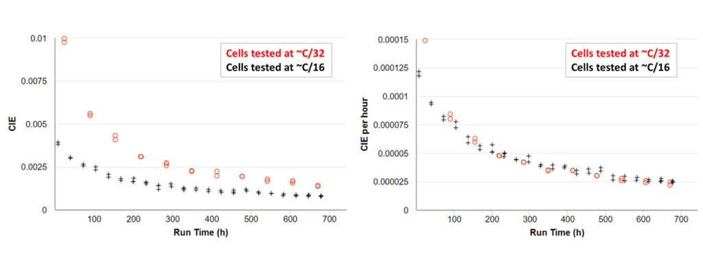
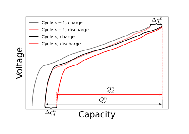
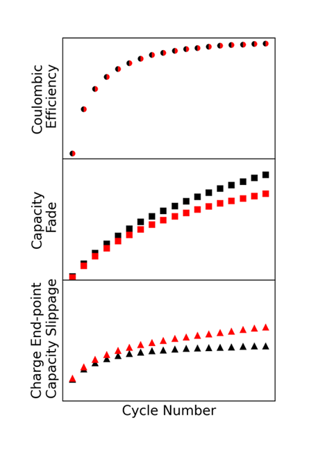
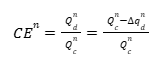
Figure 11 shows fictional data that has been modified to exaggerate both Capacity Fade and Charge Endpoint Capacity Slippage. For a given cycle \(n\), the charge endpoint is \(q_c^{n}\), and the discharge endpoint is \(q_d^{n}\). The Discharge and Charge Endpoint Capacity Slippages are the differences between the endpoints of cycle \(n\) and cycle \(n – 1\): \( \Delta q_c^{n} = q_c^{n} – q_c^{n-1} \) and \( \Delta q_d^{n} = q_d^{n} – q_d^{n-1} \), respectively. The Capacity Fade, \(Q_f\), for cycle \(n\) is the difference between the discharge capacity of cycle \(n – 1\) and cycle \(n\): \( Q_f = Q_d^{n-1} – Q_d^{n} \). Interestingly, \(Q_f\) can also be written as the difference between the Discharge and Charge Endpoint Capacity Slippages: \( Q_f = \Delta q_d^{n} – \Delta q_c^{n} \). To see this, imagine sliding the discharge curve of cycle \(n\) to the left by an amount \( \Delta q_c^{n} \) such that the charge endpoints of cycle \(n\) and cycle \(n – 1\) lie on top of each other. The difference in discharge endpoints then gives the Capacity Fade, \(Q_f\). The CE for cycle \(n\), which is the discharge to charge capacity ratio, can now be written in terms of the Capacity Fade, \(Q_f^{n}\), and the Charge Endpoint Capacity Slippage, \( \Delta q_c^{n} \), by noting that the cycle \(n\) discharge capacity is the cycle \(n\) charge capacity minus the discharge capacity slippage, \( Q_d^{n} = Q_c^{n} – \Delta q_d^{n} \).

And, as described above, the Discharge Endpoint Capacity Slippage can be expressed in terms of the Capacity Fade and Charge Endpoint Capacity Slippage:

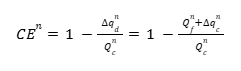
This is ultimately a very useful expression because the values \(Q_f^{n}\) and \(\Delta q_c^{n}\) can easily be extracted from cycling data for each cycle number and immediately gives insight into how the cell is degrading, whether electrolyte reduction or oxidation, for example. Before considering an example, it is worth showing how the corresponding expression for CIE per hour is obtained. The CIE is defined as \( \mathrm{CIE} = 1 – \mathrm{CE} \), and the CIE per hour is obtained by dividing by the time, \(t\), in hours, per cycle. Thus,
![]()
This expression shows that the CIE per hour can easily be obtained from the Capacity Fade and Charge Endpoint Capacity Slippage simply by normalizing each of them by the time and charge capacity per cycle.
Figure 12 shows fictional data to demonstrate the importance of interpreting data not based on CE alone, and complements the analysis discussed earlier for Figures 4 and 9. Consider a hypothetical situation where two cells have identical CE, as shown in the top panel. If no further analysis was done, one may conclude that these cells have identical electrochemical performance. However, by differentiating Capacity Fade and Charge Endpoint Capacity Slippage, it is revealed that these two cells are achieving the same CE in different ways; the cell in black has more Capacity Fade and the cell in red has more Charge Endpoint Capacity Slippage. Breaking down the CE this way and cross-referencing with other cycle metrics and experimental techniques provides additional information that can be used to make informed interpretations about how cells degrade and how chemistries can be improved, leading to higher confidence and faster decision making.
Summary
The goal of this document was to provide a foundation of knowledge for cell testing, cycle metrics, data interpretation, and an appreciation for the nuances of cycler specifications such as accuracy and precision. While not an exhaustive list of all use cases, methods, and analysis techniques, it is our hope that this document serves as a starting point to brainstorm relevant applications of UHPC for your own research and development.
For more information, visit our resource center for peer-reviewed articles, application notes, and more: https://www.novonixgroup.com/resources/
You can also visit our YouTube channel for informative webinars highlighting real experiments utilizing UHPC: https://www.youtube.com/@novonixbattery
Additionally, to learn more about the use of UHPC and to explore how it can be a valuable asset to your projects and teams, reach out to BTS-sales@novonixgroup.com.
To download a copy of the UHPC e-book, fill out the form below.
"*" indicates required fields